Model Description
The content of YoGA_Ao has been validated at several levels. This page outlines the main results.
Wavefront reconstruction models
Turbulence generation
In YoGA Ao, turbulence generation is done through extrusion of Kolmogorov-type ribbons to create an infinite phase screen (based on the work of Assémat et al, Opt. Express 14, 988–999 (2006) and Fried & Clark, J. Opt. Soc. Am. A 25, 463-468 (2008)) This process allows to generate infinite length phase screens on reasonably-sized supports. The generated screens have an infinite external scale.
Algorithm validation on the CPU
The algorithm has been first validated on the CPU. The following figure demonstrates the validity of the model by comparing the phase structure function (computed as the average of the square of each phase screen realization minus its value at pixel [1,1]) obtained on phase screens with various sizes and the theoretical value of 6.88 (r/r0)5/3.

legend: black: theoretical, red: 64x64 phase screen, blue: 80x80, green: 128x128 and yellow: 256x256.
In these simulations, the total r0 has been taken as 0.16m, a typical value at 0.5µm for a professional astronomical site. A minimum of 100,000 column extrusion is required to get a good convergence. Even with such a number of iterations, the figure above shows that the larger the screen is the slower is convergence.
Multi-layer validation on the GPU
The algorithm has then been validated on the GPU. YoGA_Ao provides the ability to simulate several turbulent layers at various altitude and with various r0 and wind speeds and directions. On the GPU, the overall model includes phase screen generation and raytracing through each layer along a specific direction.
In this configuration, two separate targets were simulated, located at two different positions on the sky. To accommodate for the induced field of view, non-zero altitude screens have to be proportionately larger than the ground layer screen. The following figures demonstrates the validity of this model for different atmosphere configuration (for 1 layer, 4 layers, 12 layers). As a reference, the single-layer CPU result for the same total r0 (i.e. as seen from the ground) is plotted in red, the GPU result is in green.

legend: left: one layer, center: 4 layers, right: 12 layers
The discrepancies in the multi-layer cases and the theoretical structure function can at least partly be attributed to the presence of larger phase screens at altitudes > 0. As seen previously larger screens are slower to converge. Moreover this effect is only visible for low spatial frequencies which are as well the slowest to converge.
Wavefront sensor model
General model
LGS spot model
LGS cone effect
The cone effect, due to the finite height of the sodium layer where the LGS is produced, is taking into account in the simulation thanks to a GPU parallelized raytracing algorithm. For each pixel of the phase screen seen by the WFS, we calculate the sum of the corresponding pixels on each phase screen of the atmosphere layers. Each term is weighting by a the Cn² coefficient of its atmosphere layer. A linear interpolation is performed between the 4-near pixels of the atmosphere layer seen by the pixel of the WFS phase screen. Basically, this is equivalent to do a "zoom" on each phase screen and summating them.
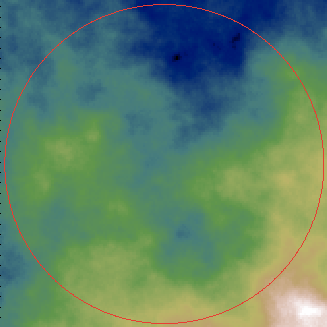
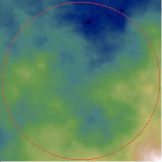
legend : first : atmosphere layer phase screen at 10km ; second : corresponding phase screen seen by the WFS with the LGS at 90km
Glenn A. Taylor has determined an analytical expression for the mean-square residual wave-front distortion E² due to the cone effect (1994, Rapid evaluation of d0 : the effective diameter of a laser guide star adaptive optics system) :
E² = (D/d0) (5/3)
where D is the telescope diameter and d0 is a measure of the effective diameter of the compensated imaging system (i.e., a telescope with a diameter equal to d0 will have 1 rad of rms wave-front error).
In order to validation our implementation of the cone effect, we suppose a system with D=4.2 m, 8x8 sub-apertures and a LGS at 90 km. We compute the variance distortion between a phase screen from a NGS and the phase screen from the LGS, and we compare it to the Taylor formula. The following figure shows the results obtained with the algorithm are in good agreement with Taylor theoretical expression: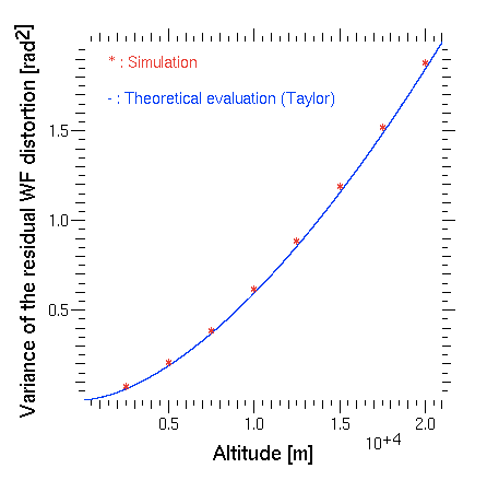
Wavefront reconstruction models
Geometric
A geometric reconstructor has been added to COMPASS : it is basically a projection of the incident phase on the DM actuators.
More details, see geometric controller document
See permormances in Benchmark results
Minimum variance
The minimum variance reconstructor aims to minimize the variance of the difference between the estimated phase and the real one. If the statistical variables are gaussian, this is equivalent to a Maximum A Priori (MAP) approach where we want to maximize the probability of obtaining such measures knowing the phase. By solving this problem, the reconstructor can be written as :
R = Cφ * D t * (D*Cφ*D t + Cn) -1
where Cφ is the phase covariance matrix, D is the DM interaction matrix (D t is its transpose) and Cn the noise matrix.
Considering that D t*Cphi*D is equivalent to the measurements covariance matrix Cmm, we can rewrite the reconstructor as :
R = Cφm * Cmm -1
where Cφm is a covariance matrix between the phase and the DM actuators
Cφm and Cmm are computed from the same way described by Eric Gendron et al. in "A novel fast and accurate pseudo-analytical simulation approach for MOAO"
Then, the reconstructor allows to compute the command matrix and the DM commands are computed thanks to Pseudo-Open Loop Control equations using the interaction matrix and previous commands to estimate open loop measurements from the closed loop one.
See permormances in Benchmark results
Mis à jour par Florian Ferreira il y a environ 11 ans · 11 révisions